
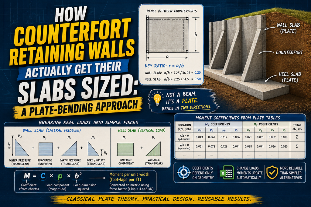
If you’ve ever looked at a counterfort retaining wall—one of those tall walls with triangular buttresses (counterforts) spaced along the back—you might assume the wall slab and heel slab are designed the same way as a simple cantilever beam. They don’t. Because the counterforts brace the slabs on the sides, each panel behaves more like a plate supported on three edges and free on the fourth, not a simple one-way strip. That distinction is why this design method exists, and it’s worth understanding before you ever open a spreadsheet.
The problem with treating slabs as beams
A wall slab spanning between two counterforts, or a heel slab spanning between the same counterforts underneath the backfill, is restrained along the two vertical (or horizontal) edges where it meets the counterforts, and along the bottom or back edge where it meets the base or stem. The remaining edge is unsupported. Loaded this way, the slab bends in two directions at once — moments vary across both the x and y axes of the panel, not just along one span.
Solving that kind of two-way bending by hand, for every combination of panel proportions and load shapes, isn’t practical. So engineers rely on precomputed moment coefficients — tables (originally derived from classical plate-bending theory, popularized in charts like Moody’s) that give the moment at any point on a rectangular plate, for a given edge-support condition, a given ratio of the plate’s short side to long side, and a given load pattern.
The key ratio: r = a/b
Every plate-coefficient table is built around one governing ratio:
r = a / b
where a is the panel’s shorter dimension (the counterfort spacing, in this case) and b is the longer dimension (the panel height or width). This ratio alone determines how the load spreads between the supported edges — a nearly square panel (r close to 1) behaves very differently from a long, narrow one (r close to 0).
In the worked example this spreadsheet is based on:
- The wall slab panel has a/b = 7.25 ft / 36.25 ft = 0.2 — a long, narrow panel, so most of the load runs down toward the base rather than across to the counterforts.
- The heel slab panel has a/b = 7.25 ft / 14.5 ft = 0.5 — closer to square, so the load splits more evenly.
Because published charts only tabulate coefficients at specific r values, getting r = 0.2 or 0.5 exactly (rather than needing to interpolate between chart lines) is what makes this particular example clean to reproduce.
Breaking a messy load into simple pieces
Real loading on a retaining wall panel is anything but simple: earth pressure that grows with depth, a surcharge that’s constant, water pressure limited to a shallow zone, and pore/uplift pressure with its own distribution. None of that matches a single “textbook” load case on its own.
The trick is superposition. Because the plate is linear-elastic, you can split the real load into several idealized components — each one a shape that already has a published coefficient table (uniform load, triangular load, etc.) — solve each one separately, and add the results.
For the wall slab, the actual lateral pressure is decomposed into four components:
- p_w — water pressure, a triangle confined to the upper portion of the wall
- p_q — surcharge pressure, uniform over the full height
- p_e — earth pressure, a triangle increasing over the full height
- p_s — pore/uplift pressure, a triangle over the lower portion
For the heel slab, the net vertical load (weight of soil and surcharge above, minus buoyant relief) is split into just two components:
- p_u — a uniform component
- p_v — a variable (triangular) component
Each component gets its own moment coefficient at every point of interest, and the total moment at that point is simply the sum of the individual contributions — which is exactly why the spreadsheet has one coefficient column per load component instead of one combined column.
From coefficient to actual moment
For a given point on the panel (located by its position as fractions of the span, x/a and y/b), the chart gives a dimensionless coefficient. The moment at that point is:
M = coefficient × p × b²
where p is the magnitude of that load component and b is the long dimension of the panel. This is the standard convention in these classical plate tables: the result is a moment per unit width of the panel (traditionally reported in foot-kips per foot of width, with the “per foot” left implicit) — which is also why, when the workbook was converted from imperial to metric units, the conversion used the plain force factor (1 kip = 4.448 kN) rather than the length-inclusive foot-kip-to-kN·m factor. It’s a subtlety that’s easy to trip over if you’re converting these classical tables to SI by hand.
Because several load components act on the same panel, the practical step is to compute p·b² once for each component (a fixed number for a given geometry and load), then multiply by whatever coefficient applies at each (x/a, y/b) location, and sum across components for the total moment at that point.
Reading the moment tables
The moment tables (Tables 3–6 in the worked example) are organised by location along the edges of the panel:
- Points with y/b varying, x/a = 0 trace the moment along one supported edge.
- Points with x/a varying, y/b = 0 trace the moment along the perpendicular edge.
Two moment directions are tabulated separately — M_x (bending about the x-axis) and M_y (bending about the y-axis) — because a two-way plate bends differently in each direction, and both need to be checked for reinforcement design.
Reading down a wall slab table, for example, you’ll typically see the moment build up from zero at a free or lightly-loaded location to a peak somewhere along the fixed edge, then taper off — the shape you’d expect from a plate that’s picking up more restraint (and more moment) as you move toward its fixed corner.
Why this matters for design
The upshot of this whole exercise is that each moment value in the tables becomes a required reinforcement moment for that location on the slab — the numbers feed directly into flexural steel design (As = M / (φ·fy·jd), or whichever method your code uses). Because the coefficients only depend on geometry (the r ratio and the point location), while the loads depend on soil, water table, and surcharge assumptions, this two-stage structure — fixed coefficients from the chart × variable, job-specific loads — is exactly what makes the method reusable: change your backfill unit weight or your water table elevation, and every moment in the table updates without touching the coefficients at all. That’s the same separation the spreadsheet mirrors: geometry and coefficients stay put, loads flow in from project-specific inputs, and the moments recompute automatically.
The honest caveat
This method is an idealisation, and the original design guidance says so directly: real wall and heel slabs vary in thickness, and the heel slab is often quite thick relative to its short span — both of which technically violate the constant-thickness, thin-plate assumptions the coefficients are built on. The justification for using them anyway is pragmatic: for this kind of geometry, the results are still considered more reliable than the alternatives available for hand calculation. It’s a reminder that even “chart-based” structural methods carry embedded assumptions worth knowing about, not just numbers to look up.
Download the Excel sheet: Counterfort Retaining Walls
This post explains the methodology behind a counterfort retaining wall moment calculation based on classical plate-bending coefficients (the Moody’s chart approach). The accompanying spreadsheet implements the same load-decomposition and coefficient-lookup structure described here, with formulas that recompute automatically when geometry or load inputs change

D Singha is a Civil Engineer with expertise in bridge design, structural engineering, and infrastructure projects. He shares insights on engineering, construction practices, technology, and professional development.